Models & Results
Hidden Markov Model
Hidden Markov Model (HMM) is a statistical model to predict the next value based on the sequence of the previous states. It uses the Markov chain which is a sequence of possible events where the probability of each event only depends on the state attained in the previous event. [13] It also uses Output Independence which is the probability of observing an event relies on the state that directly produced this event. [14] To be able to mimic this, we create a transition and emission matrix.
Transition Matrix
A transition matrix consists of the probabilities of going from one executable to another. For example the probability of the user going from chrome.exe to cmd.exe can be calculated as shown below.

Emission Matrix
An emission matrix consists of the probabilities of going from one executable to another app or tab. For example the probability of the user going from chrome.exe to google docs can be calculated as shown below.

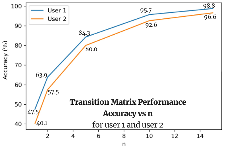
In this model, we first split the data into training and testing sets - each representing 80% and 20% of the entire dataset, respectively. We then input these data into our program that learns the Markov chain and creates a transition matrix as shown below. Once we train the data on our training set, we then run it on our test set and calculate the accuracy of the model. To calculate the accuracy, we decide if the prediction is considered accurate as long as the prediction falls in the top n probabilities for that application. As the value of n increases, the prediction accuracy increases as well.

Results
The accuracy of HMM models is calculated based on whether or not the prediction falls in the top n probabilities for that application. As the value of n (the number of applications) increases, the prediction accuracy increases as well. However, when reaching a particular value of n such as n = 10, the amount of accuracy increase starts to plateau and does not fluctuate much. Continuing to increment n won’t produce new interesting results or help us visualize the significant increase in the transition matrix’s accuracy. Thus, we conclude the optimal n should be n = 5 in our case.

Long Short-term Memory Model
The Long Short-Term Memory (LSTM) model is a type of recurrent neural network (RNN) that is designed to overcome the vanishing gradient problem, which is a common issue with traditional RNNs. LSTMs are widely used in natural language processing, speech recognition, and image recognition tasks.
Memory Cells
At the core of the LSTM model are memory cells, which can store information for a long time. The model uses a combination of three gates - input, forget, and output gates - to regulate the flow of information into and out of the memory cells. The input gate controls how much new information is added to the memory cells, the forget gate determines which information is removed from the memory cells, and the output gate controls how much information is read from the memory cells.
Cell State
The LSTM model also has a cell state that runs along with the memory cells. The cell state carries information across different time steps and can be modified through the use of the gates. The model's ability to selectively add or remove information from the memory cells and cell state, as well as its ability to remember information over long periods of time, makes it well-suited for handling sequential data.
Training + Back Propagation
During the training process, the model learns to optimize the weights of the gates and memory cells through backpropagation, where the error from the output is propagated back through time. This allows the model to make more accurate predictions over time as it learns to capture the patterns and relationships in the input data..
Applying this model to our collected data proved to provide very powerful insights. Using the collected data and some data manipulation, we are capable of tackling two prediction problems:
- Predict the duration a user spends on an app within an hour, given the past time-series data.
- Predict the total amount of time a particular user spends using a particular app on any given day.
Results
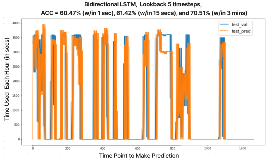
After trying different models and feature engineering techniques, we conclude that the Bidirectional LSTM provides the best possible result for our first prediction problem. It can capture both the peaks and the low values of the time usage as shown in the figure below. In fact, the bidirectional characteristics allow the model to learn in both forward and backward directions. [17]

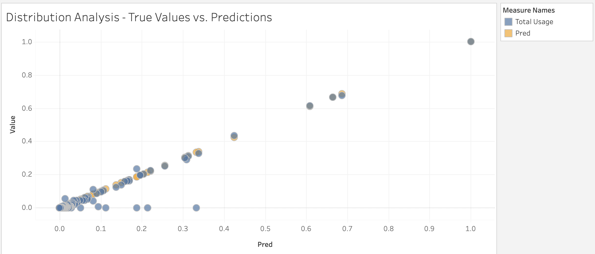
As for the second prediciton problem. We use a different model consisting of the usage time used of each application in a day split into each hour of the day, the total usage of that app during that day, and a value to differentiate each application. Using this model, we make predictions on the total usage. The prediction values are continuous in nature. Thus, to properly understand the accuracy of the model a binning process was conducted based on thresholds that were determined through analysis of the distribution of the true and predicted values. The distribution of these values can be seen below. Through the binning process we were able to determine that the model performs at about 70% accuracy.
